PyPlot
Raccolta di esempi, esercizi, snippets.
Matplot : python library for graph plotting.
Matplot tutorials : some tutorials
sudo apt install python-matplotlib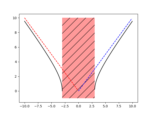
sudo apt install python3-matplotlibThe following function is plotted highlighting asymptotes and domains area
\( y = \sqrt{(x^2 - 9)} \)
Herebelow the python code:
import numpy as np
import matplotlib.pyplot as plt

x = np.arange(-10, 10, 0.01)

y = (x**2 - 9)**(0.5)
plt.plot(x,y,'black')

x1 = np.arange(0 , 10, 0.1)
asintoto1 = x1
x2 = np.arange(-10 , 0, 0.1)
asintoto2 = -x2
plt.plot(x1,asintoto1,color='b',linestyle='dashed')
plt.plot(x2,asintoto2,color='r',linestyle='dashed')

xfill = [-3, -3,  3,  3]
yfill = [-1, 10, 10, -1]
# alpha = tranparency (real)
# hatch = filling pattern
plt.fill(xfill,yfill,'r', alpha=0.4 , hatch='/')

plt.savefig("plot_func1.png")
plt.show()
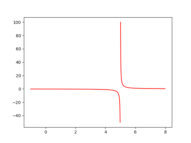
The following function is plotted to avoid singularity
\( y = { 1 \over { x-5 } } \)
Herebelow the python code:
import numpy as np
import matplotlib.pyplot as plt

x1 = np.arange(5.01, 8, 0.01)
x2 = np.arange(-1, 4.99, 0.01)


y1 = 1 / (x1-5)
plt.plot(x1,y1,'red')

y2 = 1 / (x2-5)
plt.plot(x2,y2,'red')


plt.savefig("plot_func2.png")
plt.show()
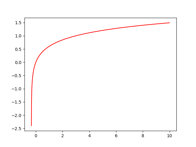
The following function is plotted to show a logariithmic function
\( y = log(3x+1) \)
Herebelow the python code:
import numpy as np
import matplotlib.pyplot as plt

x = np.arange(-0.332, 10, 0.01)

y = np.log10(3*x+1)
plt.plot(x,y,'red')

plt.savefig("plot_func3.png")
plt.show()
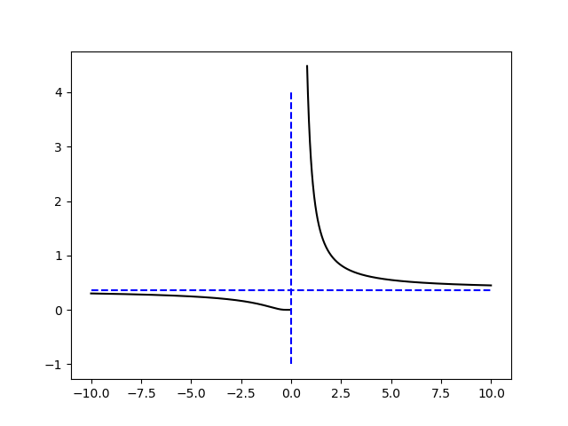
The following function is plotted to show a exponential function
\( y = \exp \left( { { 2-x } \over x } \right) \)
Herebelow the python code:
import numpy as np
import matplotlib.pyplot as plt


xa = np.arange(-10, -0.01, 0.01)

ya = np.exp( ( 2-xa ) / xa )
plt.plot(xa,ya,'black')

xb = np.arange(0.8, 10, 0.01)

yb = np.exp( ( 2-xb ) / xb )
plt.plot(xb,yb,'black')


x1 = [ -10 , 10 ]
asintoto1 = [ np.exp(-1) , np.exp(-1) ]
plt.plot(x1,asintoto1,color='b',linestyle='dashed')

x2 = [ 0 , 0 ]
asintoto2 = [ -1 , 4 ]
plt.plot(x2,asintoto2,color='b',linestyle='dashed')


plt.savefig("plot_func4.png")
plt.show()
The following function is plotted to show a sinusoidal function and image type ong and svg.
\( y = \sin(x) \)
PNG image:
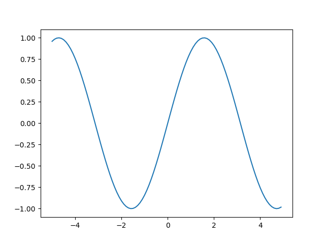
SVG image:

Herebelow the python code:
import numpy as np
import matplotlib.pyplot as plt


xa = np.arange(-10, -0.01, 0.01)

ya = np.exp( ( 2-xa ) / xa )
plt.plot(xa,ya,'black')

xb = np.arange(0.8, 10, 0.01)

yb = np.exp( ( 2-xb ) / xb )
plt.plot(xb,yb,'black')


x1 = [ -10 , 10 ]
asintoto1 = [ np.exp(-1) , np.exp(-1) ]
plt.plot(x1,asintoto1,color='b',linestyle='dashed')

x2 = [ 0 , 0 ]
asintoto2 = [ -1 , 4 ]
plt.plot(x2,asintoto2,color='b',linestyle='dashed')


plt.savefig("plot_func4.png")
plt.show()
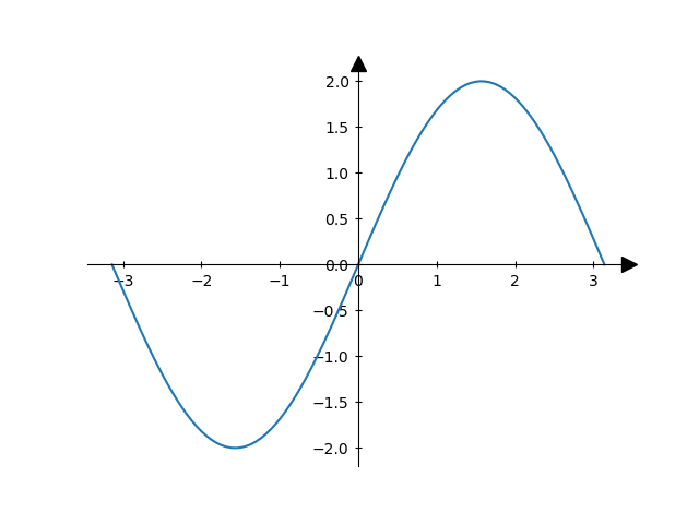
From this, a classical math-style graph
Herebelow the python code:
import numpy as np
import matplotlib.pyplot as plt


x = np.linspace(-np.pi, np.pi, 100)
y = 2 * np.sin(x)

rc = {"xtick.direction" : "inout", "ytick.direction" : "inout",
      "xtick.major.size" : 5, "ytick.major.size" : 5,}

with plt.rc_context(rc):
    fig, ax = plt.subplots()
    ax.plot(x, y)

    ax.spines['left'].set_position('zero')
    ax.spines['right'].set_visible(False)
    ax.spines['bottom'].set_position('zero')
    ax.spines['top'].set_visible(False)
    ax.xaxis.set_ticks_position('bottom')
    ax.yaxis.set_ticks_position('left')

    # make arrows
    ax.plot((1), (0), ls="", marker=">", ms=10, color="k",
            transform=ax.get_yaxis_transform(), clip_on=False)
    ax.plot((0), (1), ls="", marker="^", ms=10, color="k",
            transform=ax.get_xaxis_transform(), clip_on=False)


plt.savefig("plot_func6.png")
plt.show()
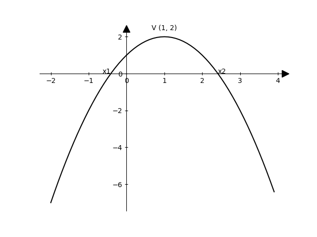
Label points
Herebelow the python code:
import numpy as np
import matplotlib.pyplot as plt

x = np.arange(-2, 4, 0.1)

y = - x**2 + 2*x + 1


rc = {"xtick.direction" : "inout", "ytick.direction" : "inout",
      "xtick.major.size" : 5, "ytick.major.size" : 5,}

with plt.rc_context(rc):
    fig, ax = plt.subplots()
    ax.plot(x, y, 'black')

    ax.spines['left'].set_position('zero')
    ax.spines['right'].set_visible(False)
    ax.spines['bottom'].set_position('zero')
    ax.spines['top'].set_visible(False)
    ax.xaxis.set_ticks_position('bottom')
    ax.yaxis.set_ticks_position('left')

    # make arrows
    ax.plot((1), (0), ls="", marker=">", ms=10, color="k",
            transform=ax.get_yaxis_transform(), clip_on=False)
    ax.plot((0), (1), ls="", marker="^", ms=10, color="k",
            transform=ax.get_xaxis_transform(), clip_on=False)


#plt.text(1,2,'V',horizontalalignment='center')
#plt.text(1,2,'V',horizontalalignment='center')
plt.text(-0.41,0,'x1',horizontalalignment='right')
plt.text(2.41,0,'x2',horizontalalignment='left')


xv=1
yv=2

label = "V ({0}, {1})".format(xv,yv)

plt.annotate(label, # this is the text
             (xv,yv), # this is the point to label
             textcoords="offset points", # how to position the text
             xytext=(0,10), # distance from text to points (x,y)
             ha='center') # horizontal alignment can be left, right or center


plt.savefig("plot_func7.png")
plt.show()